1 基本概念 1.1 基本问题 网络剪枝目标是
更小的模型
更快的推理(inference)速度
不对准确率精度等造成过多损失
相关技术有
权重共享
量化(quantization)
低阶近似(Low-Rank Approximation)
二元/三元网络(Binary / Ternary Net)
Winograd Transformation
1.2 当前神经网络遇到的一些挑战
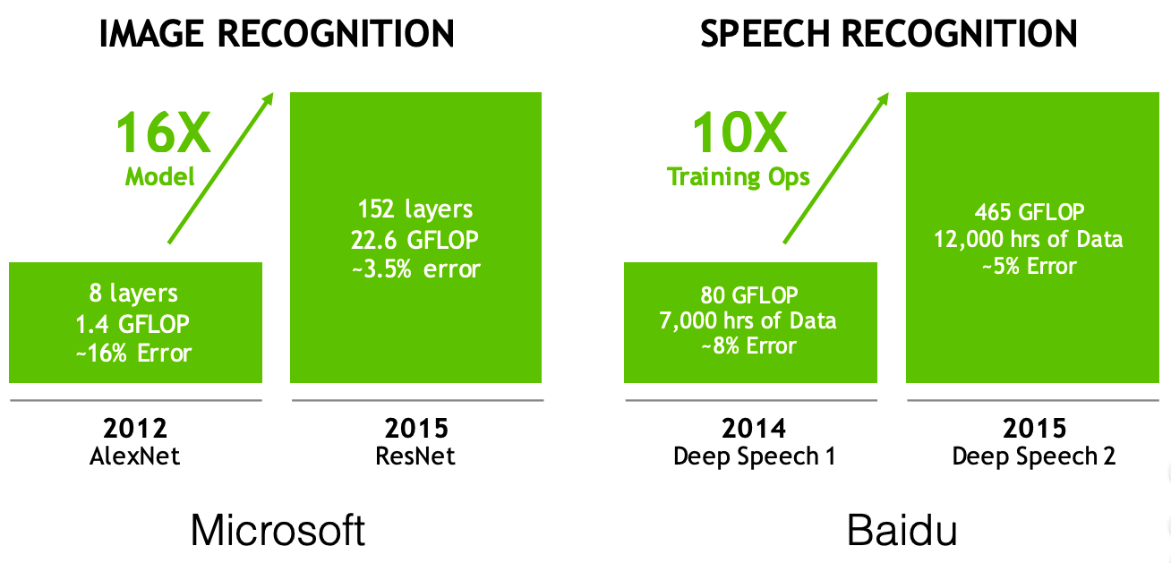
模型变得越来越大
速度越来越慢
能源效率
AlphaGo 使用了1920个CPU和280个GPU,每场比赛消耗3000美元的电力。
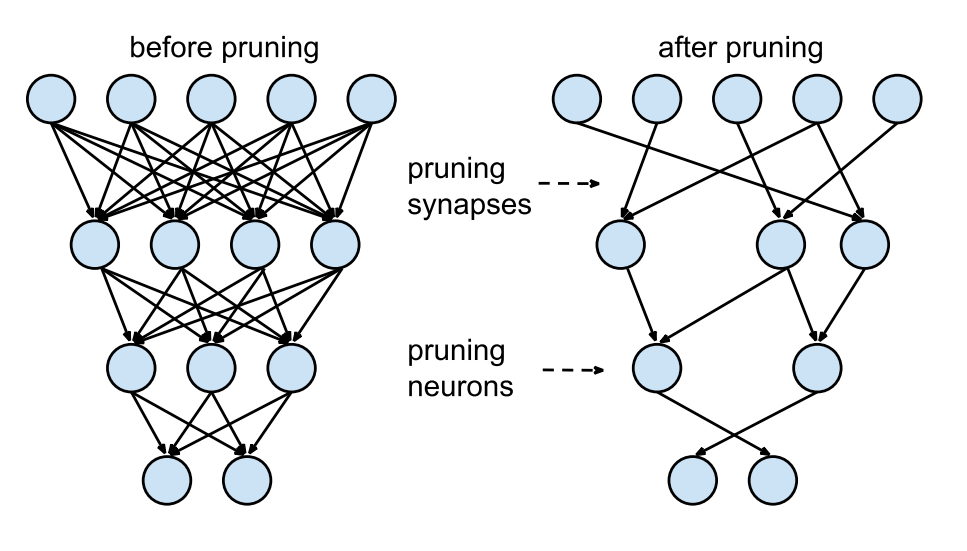
1.3 网络剪枝的原理 将原本的稠密连接网络,删去不必要的连接,变成右边相对稀疏的网络。稀疏网络易于压缩,并且可以在预测时跳过零值,提高推理速度 。
如果可以对网络的所有神经元贡献度排序,我们可以删除排在末尾的神经元,这样可就可以减小网络获得更快的推理速度。
可以使用神经元的权重的L1/L2正则来做排序。剪枝之后,准确率将会降低。通常会执行训练$\rightarrow$剪枝$\rightarrow$训练$\rightarrow$剪枝..的循环中。如果一次剪枝过多,网络可能会损坏,无法恢复。所以在实践中,这是一个迭代执行的步骤。
2 剪枝技术 2.1 权重剪枝
将权重矩阵中孤立(没有与其他权重项有连接的)的权重设置为0。这对应着上图中删除了连接
此处,为了达到k%的稀疏度,我们将孤立的权重排序。在权重矩阵中,W对应了梯度,然后将最小的k%设置为0。下面的代码演示了这个过程
1
2
3
4
5
6
7
8
9
10
11
12
f = h5py.File("model_weights.h5",'r+') for k in [.25, .50, .60, .70, .80, .90, .95, .97, .99]: ranks = {} for l in list(f[‘model_weights’])[:-1]: data = f[‘model_weights’][l][l][‘kernel:0’] w = np.array(data) ranks[l]=(rankdata(np.abs(w),method=’dense’) — 1).astype(int).reshape(w.shape) lower_bound_rank = np.ceil(np.max(ranks[l])*k).astype(int) ranks[l][ranks[l]<=lower_bound_rank] = 0 ranks[l][ranks[l]>lower_bound_rank] = 1 w = w*ranks[l] data[…] = w
2.2 神经元剪枝
将神经元对应的权重矩阵中的一整列的值全部设为0,这等同于删除了对应的输出神经元
此处,要达到k%的稀疏度,我们对权重矩阵的列排序,排序规则是它们的L2正则,然后删除最小的k%。
1
2
3
4
5
6
7
8
9
10
11
12
13
14
f = h5py.File("model_weights.h5",'r+') for k in [.25, .50, .60, .70, .80, .90, .95, .97, .99]: ranks = {} for l in list(f[‘model_weights’])[:-1]: data = f[‘model_weights’][l][l][‘kernel:0’] w = np.array(data) norm = LA.norm(w,axis=0) norm = np.tile(norm,(w.shape[0],1)) ranks[l] = (rankdata(norm,method=’dense’) — 1).astype(int).reshape(norm.shape) lower_bound_rank = np.ceil(np.max(ranks[l])*k).astype(int) ranks[l][ranks[l]<=lower_bound_rank] = 0 ranks[l][ranks[l]>lower_bound_rank] = 1 w = w*ranks[l] data[…] = w
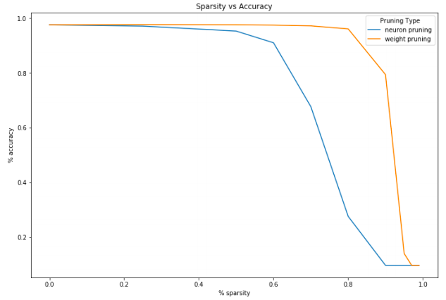
通常随着你增加稀疏度,并且删除越来越多的神经元,模型的性能会下降,此时就需要对模型性能和稀疏度作出取舍了。
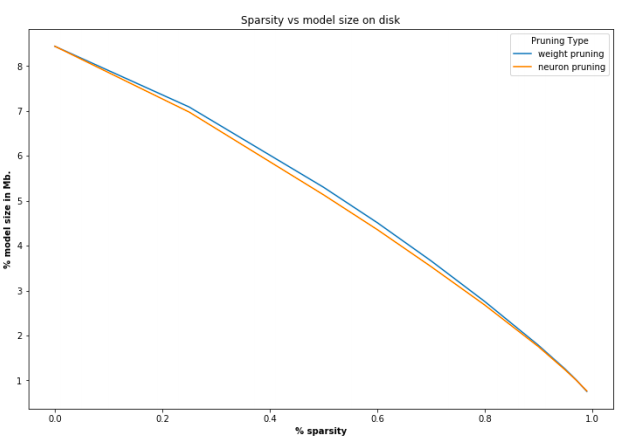
2.3 权重稀疏和神经元稀疏的对比
看起来权重稀疏更柔和一些。
权重稀疏和神经元稀疏在减小网络尺寸上效果相同。
2.4 剪枝的问题 参考自Pruning deep neural networks to make them fast and small ,说明尽管有诸多剪枝的论文,但是在现实世界里很少使用剪枝,究其原因,可能有如下
按照贡献度排序的方法目前为止上不够完善,精度损失过高
难以实现
一些公司使用了剪枝技术,但是没有公开这个秘密
3 剪枝实践 3.1 剪枝为了速度VS为了更小的模型 VGG模型90%的权重在后面的全连接层,但是只贡献了1%的浮点运算。最近,人们才开始专注裁剪全连接层,通过替换全连接层模型尺寸会大幅度缩减。此处只关注于裁剪整个卷积层,但是它有个很好的副作用就是同事减小了内存消耗,如论文1611.06440 Pruning Convolutional Neural Networks for Resource Efficient Inference 所述,网络层越深,越容易被裁剪。这表明最后的卷积层会大幅度被裁剪,全连接后面的诸多神经元也会被抛弃。
对卷积层裁剪时,同时也可以对每个卷积核做权重衰减,或者移除某个卷积核的某个特定维度(列),这样会得到稀疏的卷积核,这么得来的结果无法得到计算速度的提升。最近的研究提倡结构稀疏,即整个卷积核被裁剪掉。
另外一个重要提示是通过训练然后裁剪一个大网络,尤其在迁移学习时,其结果比从头训练一个小网络要好得多
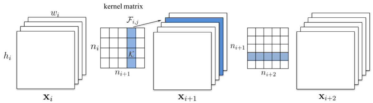
3.2 裁剪卷积核 参考论文Pruning filters for effecient convents .
此论文提倡裁剪掉整个卷积核。裁剪一个卷积核的索引k,影响的是它所在网络层,以及后续的网络层。所有在索引k处的输入通道,在后续网络层会被移除掉,如下图。
假若后续层是全连接层,以及feature map的通道的尺寸会是$M\times N$,那么将会从全连接层中移除$M\times N$个神经元。
神经元的排序相当简单,即它们每个卷积核的权重的L1 norm。
每次剪枝迭代都会对所有卷积核的权重L1 norm排序,裁剪掉末尾的m个filter,重新训练,并重复。
3.3 结构剪枝 参考论文1512.08571 Structured Pruning of Deep Convolutional Neural Networks
论文内容与上面差不多,但是排序算法复杂得多。论文使用了一个有N个粒子过滤器(particle filters)的集合,保存了N个即将被裁剪的卷积核。
如果粒子(particle)所代表的卷积核没有被mask划出,每个粒子(particle)被分配一个基于网络在验证集上准确率的得分。然后基于新的得分,会得到新的裁剪mask。
3.4 nvidia裁剪:卷积核裁剪以提升资源推理效率(Resource Efficient Inference) 参考论文1611.06440 Pruning Convolutional Neural Networks for Resource Efficient Inference 。
首先,他们提出了将一个裁剪问题视为某种优化问题:选取权重B的子集,如果裁剪它们使得网络的损失变化得最小
$$
注意:使用的是绝对值差异而非简单的差异,这样裁剪网络不会太多地缩减网络的性能,但是也应该不会增加。
这样一来,所有的排序方法可以使用此损失函数来衡量了。
3.5 Oracle裁剪 VGG16有4224个卷积核,完美的排序方法应该使用暴力裁剪每个卷积核,然后观察在训练集上损失函数变化,此方法称为oracle排序,最可能的排序方法。为了衡量其他排序方法的的效率,他们计算了其他方法与oracle的speraman协相关系数。令人惊讶的是,它们想到的排序方法(下文提到)与oracle协相关程度最高。
它们想到一个新的基于损失函数的泰勒一阶展开(代表最快的计算)神经元排序方法,裁剪一个卷积核$h$与将其清零相同。
$C(W,D)$是网络权重被设为W时在数据集D上的平均损失。现在,我们可以评估$C(W,D)$的在$C(W,D,h=0)$处的展开,它们 应该十分相近,因为移除单一卷积核不会对损失值造成太大影响。
$h$的排序为$C(W,D,h=0)-C(W,D)$的绝对值。
$${TE}(h_i)=|\triangle C(h_i)|=|C(D,h_i)-\frac{\partial C}{\partial h_i}h_i-C(D,h_i)|=|\frac{\partial C}{\partial h_i}h_i|\{TE}(z_l ^{k})=|\frac{1}{M}\sum_m \frac{\partial C}{\partial z {l,m} ^{(k)}}z {l,m} ^{(k)}
每一层的排序都会那一整层的排序的L2 norm的排序再次normalized。这有点经验主义,不太确定是否真有必要,但是极大地影响剪枝质量。
这种排序是相当直觉性的,我们不能同时使用排序方法本身所使用的激活函数、梯度。如果(激活函数、梯度)任意一个很高,代表其对输出有较大影响。将它们相乘,根据梯度或者激活函数值非常高或低,可以让我们得以衡量,是抛弃还是继续保留该卷积核。
这让我很好奇,他们到底有没有将剪枝问题视为最小化网络损失函数值差异,然后想出的泰勒展开式,还是说相反的,网络损失值差异是他们的某种备份的新方法。
4 剪枝实践:对一个猫狗二分类器裁剪,使用泰勒展开式为排序准则 使用1000张狗和1000张猫的图片,对VGG模型做迁移学习训练。猫狗图片来自kaggle猫狗分类 ,使用400张猫和400张狗的图片作为测试集。
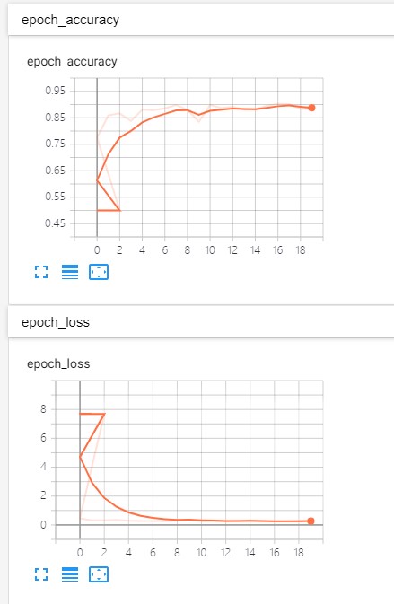
4.1 剪枝之后的结果说明
准确率从98.7%掉到97.5%
网络模型从538MB减小到150MB
在i7 CPU上推理时间从0.78秒减小到0.227秒。基本是原来的三分之一
4.2 第一步:训练一个大网络 使用一个VGG16,然后丢弃最后三个全连接层,然后添加新的三个全连接层,此过程会freeze所有的卷积层,只训练新的三个全连接层。
我们先准备数据集,从kaggle下载数据之后,从总分别选取1400张猫和1400张狗,其中1000张猫和1000张狗作为训练集,放在train1000目录下的cat和dog目录下,另外的400张猫和400张狗放在val目录下的cat和dog目录下。使用Tensorflow2.0的代码示例如下
1
2
3
4
5
6
7
8
9
10
11
12
13
14
15
16
17
18
19
20
21
22
23
24
25
26
27
28
29
30
31
32
33
34
35
36
37
38
39
40
41
42
43
44
45
46
47
48
49
50
51
52
53
54
55
56
57
58
59
60
61
62
63
64
65
66
67
68
69
70
71
72
73
74
75
76
77
78
79
80
81
82
83
84
85
86
87
88
89
90
91
92
93
94
95
96
97
98
99
100
101
102
103
104
105
106
107
108
109
110
111
112
113
import os import tensorflow as tf from keras_applications.vgg16 import VGG16 from tensorflow.keras.preprocessing.image import ImageDataGenerator from tensorflow.keras.optimizers import Adam from tensorflow.keras.callbacks import TensorBoard,ModelCheckpoint,ReduceLROnPlateau,Callback ## global parameters lr = 1e-4 input_width,input_height = 224,224 weight_save_path = "./vgg16_catdog_weights/" record_save_path = "./vgg16_catdog_tensorboard/" model_weight_file = weight_save_path + "vgg16_catdog_binary.h5" optimizer = Adam(lr=0.0001, beta_1=0.9, beta_2=0.999, epsilon=1e-08) # Callback for early stopping the training early_stopping = tf.keras.callbacks.EarlyStopping(monitor='val_accuracy', min_delta=0, patience=15, verbose=1, mode='auto') # set model checkpoint callback (model weights will auto save in weight_save_path) checkpoint = ModelCheckpoint(model_weight_file, monitor='val_accuracy', verbose=1, save_best_only=True, mode='max', period=1) # monitor a learning indicator(reduce learning rate when learning effect is stagnant) reduceLRcallback = ReduceLROnPlateau(monitor='val_acc', factor=0.7, patience=5, verbose=1, mode='auto', cooldown=0, min_lr=0) class LossHistory(Callback): def on_train_begin(self, logs={}): self.losses = [] self.val_losses = [] self.acc = [] self.val_acc = [] self.recall = [] def on_epoch_end(self, batch, logs={}): self.losses.append(logs.get('loss')) self.val_losses.append(logs.get('val_loss')) self.acc.append(logs.get('acc')) self.val_acc.append(logs.get('val_accuracy')) self.recall.append(logs.get('recall')) def build_model(input_width,input_height,drop_prob=0.5): vgg = VGG16(include_top=False,weights="imagenet",classes=2,input_shape=(input_width,input_height,3),backend = tf.keras.backend, layers = tf.keras.layers, models = tf.keras.models, utils = tf.keras.utils) for layer in vgg.layers: layer.trainable =False print(vgg.summary()) out = tf.keras.layers.Flatten()(vgg.output) dense1 =tf.keras.layers.Dense(4096,activation="relu")(out) drop1 = tf.keras.layers.Dropout(drop_prob)(dense1) dense2 =tf.keras.layers.Dense(4096,activation="relu")(drop1) drop2 = tf.keras.layers.Dropout(drop_prob)(dense2) dense3 =tf.keras.layers.Dense(1,activation="sigmoid")(drop2) merged_model = tf.keras.models.Model(vgg.input,dense3) print(merged_model.summary()) return merged_model def train_val_generator(train_img_path,val_img_path): train_datagen = ImageDataGenerator(rescale=1 / 255., rotation_range=45, width_shift_range=0.2, # degree of horizontal offset(a ratio relative to image width) height_shift_range=0.2, # degree of vertical offset(a ratio relatice to image height) shear_range=0.2, # the range of shear transformation(a ratio in 0 ~ 1) zoom_range=0.25, # degree of random zoom(the zoom range will be [1 - zoom_range, 1 + zoom_range]) horizontal_flip=True, # whether to perform horizontal flip vertical_flip=True, # whether to perform vertical flip fill_mode='nearest' # mode list: nearest, constant, reflect, wrap ) val_datagen = ImageDataGenerator(rescale=1 / 255.) train_generator = train_datagen.flow_from_directory( train_img_path, shuffle=True, target_size=(input_width,input_height), batch_size=batch_size, class_mode='binary') validation_generator = val_datagen.flow_from_directory( val_img_path, target_size=(input_width,input_height), batch_size=batch_size, class_mode='binary') return train_generator,validation_generator def train_model(train_img_path,val_img_path,batch_size,epochs): if os.path.exists(model_weight_file): model = tf.keras.models.load_model(model_weight_file) else: model = build_model(input_width,input_height) model.compile(optimizer=optimizer, loss='binary_crossentropy', metrics=['accuracy']) train_generator, validation_generator = train_val_generator(train_img_path,val_img_path) train_sample_count = len(train_generator.filenames) val_sample_count = len(validation_generator.filenames) print(train_sample_count, val_sample_count) history = LossHistory() model.fit_generator( train_generator, steps_per_epoch=int(train_sample_count / batch_size) + 1, epochs=epochs, validation_data=validation_generator, validation_steps=int(val_sample_count / batch_size) + 1, callbacks=[TensorBoard(log_dir=record_save_path), early_stopping, history, checkpoint, reduceLRcallback] ) if __name__== '__main__': train_set_path = 'E:/data/images/dogs-vs-cats/train1000' valid_set_path = 'E:/data/images/dogs-vs-cats/val' batch_size = 8 epochs = 20 train_model(train_set_path, valid_set_path, batch_size,epochs)
最后的准确率,没有作者那么高,只有90%,如下:
1
2
3
4
5
6
7
8
9
10
11
12
13
14
15
16
17
18
236/251 [===========================>..] - ETA: 2s - loss: 0.3744 - accuracy: 0.8231 237/251 [===========================>..] - ETA: 2s - loss: 0.3738 - accuracy: 0.8233 238/251 [===========================>..] - ETA: 2s - loss: 0.3747 - accuracy: 0.8230 239/251 [===========================>..] - ETA: 1s - loss: 0.3746 - accuracy: 0.8232 240/251 [===========================>..] - ETA: 1s - loss: 0.3746 - accuracy: 0.8229 241/251 [===========================>..] - ETA: 1s - loss: 0.3747 - accuracy: 0.8231 242/251 [===========================>..] - ETA: 1s - loss: 0.3738 - accuracy: 0.8239 243/251 [============================>.] - ETA: 1s - loss: 0.3735 - accuracy: 0.8236 244/251 [============================>.] - ETA: 1s - loss: 0.3728 - accuracy: 0.8243 245/251 [============================>.] - ETA: 0s - loss: 0.3728 - accuracy: 0.8240 246/251 [============================>.] - ETA: 0s - loss: 0.3718 - accuracy: 0.8242 247/251 [============================>.] - ETA: 0s - loss: 0.3735 - accuracy: 0.8239 248/251 [============================>.] - ETA: 0s - loss: 0.3746 - accuracy: 0.8231 249/251 [============================>.] - ETA: 0s - loss: 0.3745 - accuracy: 0.8228 250/251 [============================>.] - ETA: 0s - loss: 0.3736 - accuracy: 0.8235 Epoch 00020: val_accuracy did not improve from 0.90274 251/251 [==============================] - 47s 188ms/step - loss: 0.3742 - accuracy: 0.8227 - val_loss: 0.2761 - val_accuracy: 0.8815
查看对应的验证集的tensorboard如下
4.3 对卷积核排序 为了计算泰勒展开指标,我们需要在数据集上做一个前向+后向传播(可以在一个较小的数据集上)。
现在需要获取卷积层的梯度和激活函数。可以在梯度计算时注册一个hook,当这些东西就绪时会调用这个callback。
现在,我们可以从self.activations中获得激活函数值,当梯度就绪时会执行计算排序的方法
1
2
3
4
5
6
7
8
9
10
11
12
13
14
15
16
17
def compute_rank(self, grad): activation_index = len(self.activations) - self.grad_index - 1 activation = self.activations[activation_index] values = \ torch.sum((activation * grad), dim = 0).\ sum(dim=2).sum(dim=3)[0, :, 0, 0].data # Normalize the rank by the filter dimensions values = \ values / (activation.size(0) * activation.size(2) * activation.size(3)) if activation_index not in self.filter_ranks: self.filter_ranks[activation_index] = \ torch.FloatTensor(activation.size(1)).zero_().cuda() self.filter_ranks[activation_index] += values self.grad_index += 1
5. 剪枝实践:使用Tensorflow 训练剪枝MNIST模型为例 下面使用tensorflow api为例,其他API也有类似功能。基于keras api的权重剪枝,在训练过程中迭代的删除一些没用的连接,基于连接的梯度。下面示范通过简单的使用一种通用文件压缩算法(如zip压缩),就可以缩减keras模型
5.1 训练一个剪枝的模型 tensorflow提供一个prune_low_magnitude()的API来训练模型,模型中会移除一些连接。基于Keras的API可以应用于独立的网络层,或者整个网络。在高层级,此技术是在给定规划和目标稀疏度的前提下,通过迭代的移除(即zeroing out)网络层之间的连接。
例如,典型的配置是目标稀疏度为75%,通过每迭代100步(epoch)裁剪一些连接,从第2000步(epoch)开始。更多配置需要查看官方文档。
5.2 一层一层的构建一个剪枝的模型 下面展示如何在网络层层面使用API,构建一个剪枝的分类模型。
此时,prune_low_magnitude()接收一个想要被裁剪的网络层作为参数。
此函数需要一个剪枝参数,配置的是在训练过程中的剪枝算法。以下是相关参数的意义
Sparsity : 整个训练过程中使用的是多项式递减(PolynomialDecay)。从50%的稀疏度开始,然后逐渐地训练模型以达到90%的稀疏度。x%的稀疏度代表x%的权重标量将会被裁剪掉Schedule :从第2000步开始到训练结束,网络层之间的连接会逐渐被裁剪掉,并且是每100步执行一次。究其原因是,要训练一个在几个步骤内稳定达到一定准确率的模型,以帮助其收敛。同时,也让模型在每次裁剪之后能恢复,所以并不是每一步都要裁剪。我们可以将裁剪频率设为100.
为了演示如何保存并重新载入裁剪的模型,我们先训练一个模型10个epoch,保存,然后载入模型并继续训练2个epoch。逐渐地稀疏,四个重要参数是**begin_sparsity,final_sparsity,begin_step,end_step**。
1
2
3
4
5
6
7
8
9
10
11
12
13
14
15
16
17
18
19
20
21
22
23
24
25
26
27
28
29
30
31
32
from tensorflow_model_optimization.sparsity import keras as sparsity epochs = 12 l = tf.keras.layers num_train_samples = x_train.shape[0] end_step = np.ceil(1.0 * num_train_samples / batch_size).astype(np.int32) * epochs print('End step: ' + str(end_step)) pruning_params = { 'pruning_schedule': sparsity.PolynomialDecay(initial_sparsity=0.50, final_sparsity=0.90, begin_step=2000, end_step=end_step, frequency=100) } pruned_model = tf.keras.Sequential([ sparsity.prune_low_magnitude( l.Conv2D(32, 5, padding='same', activation='relu'), input_shape=input_shape, **pruning_params), l.MaxPooling2D((2, 2), (2, 2), padding='same'), l.BatchNormalization(), sparsity.prune_low_magnitude( l.Conv2D(64, 5, padding='same', activation='relu'), **pruning_params), l.MaxPooling2D((2, 2), (2, 2), padding='same'), l.Flatten(), sparsity.prune_low_magnitude(l.Dense(1024, activation='relu'), **pruning_params), l.Dropout(0.4), sparsity.prune_low_magnitude(l.Dense(num_classes, activation='softmax'), **pruning_params) ]) pruned_model.summary()
作为对比,我们训练了一个MNSIT数据集的分类模型,首先,我们准备的数据和参数
1
2
3
4
5
6
7
8
9
10
11
12
13
14
15
16
17
18
19
20
21
22
23
24
25
26
27
28
29
30
31
32
33
34
35
36
37
38
39
40
41
42
43
import tensorflow as tf import tempfile import zipfile import os import tensorboard import numpy as np from tensorflow_model_optimization.sparsity import keras as sparsity ## global parameters batch_size = 128 num_classes = 10 epochs = 10 # input image dimensions img_rows, img_cols = 28, 28 logdir = tempfile.mkdtemp() print('Writing training logs to ' + logdir) def prepare_trainval(img_rows, img_cols): # the data, shuffled and split between train and test sets (x_train, y_train), (x_test, y_test) = tf.keras.datasets.mnist.load_data() if tf.keras.backend.image_data_format() == 'channels_first': x_train = x_train.reshape(x_train.shape[0], 1, img_rows, img_cols) x_test = x_test.reshape(x_test.shape[0], 1, img_rows, img_cols) input_shape = (1, img_rows, img_cols) else: x_train = x_train.reshape(x_train.shape[0], img_rows, img_cols, 1) x_test = x_test.reshape(x_test.shape[0], img_rows, img_cols, 1) input_shape = (img_rows, img_cols, 1) x_train = x_train.astype('float32') x_test = x_test.astype('float32') x_train /= 255 x_test /= 255 print('x_train shape:', x_train.shape) print(x_train.shape[0], 'train samples') print(x_test.shape[0], 'test samples') # convert class vectors to binary class matrices y_train = tf.keras.utils.to_categorical(y_train, num_classes) y_test = tf.keras.utils.to_categorical(y_test, num_classes) return x_train,x_test,y_train,y_test
5.2.1 构建原始的MNIST分类模型 使用keras构建一个简单的keras模型如下
1
2
3
4
5
6
7
8
9
10
11
12
13
14
15
16
17
18
19
20
def build_clean_model(input_shape): l = tf.keras.layers model = tf.keras.Sequential([ l.Conv2D( 32, 5, padding='same', activation='relu', input_shape=input_shape), l.MaxPooling2D((2, 2), (2, 2), padding='same'), l.BatchNormalization(), l.Conv2D(64, 5, padding='same', activation='relu'), l.MaxPooling2D((2, 2), (2, 2), padding='same'), l.Flatten(), l.Dense(1024, activation='relu'), l.Dropout(0.4), l.Dense(num_classes, activation='softmax') ]) model.compile( loss=tf.keras.losses.categorical_crossentropy, optimizer='adam', metrics=['accuracy']) model.summary() return model
训练模型代码
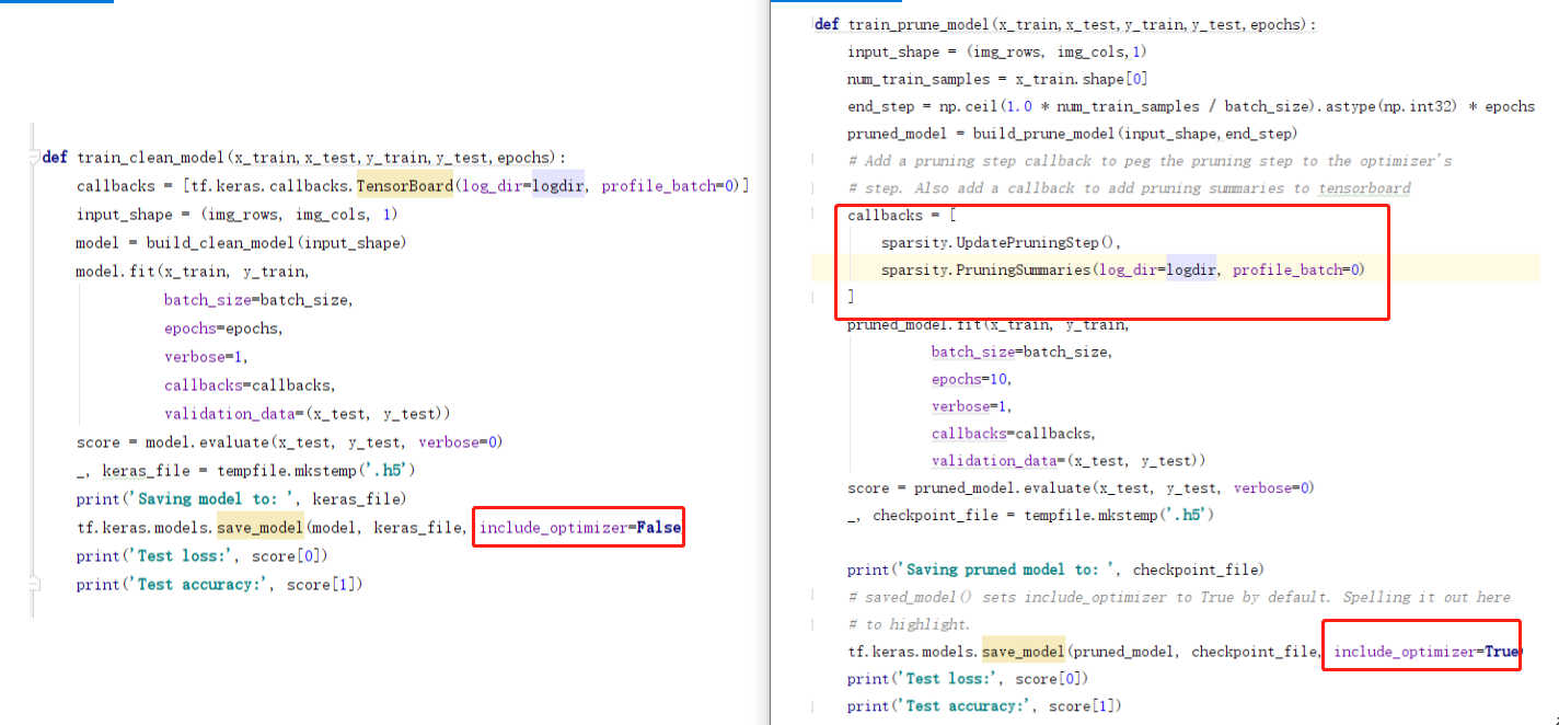
1
2
3
4
5
6
7
8
9
10
11
12
13
14
15
16
17
18
19
def train_clean_model(x_train,x_test,y_train,y_test,epochs,ori_mnist_model_file): callbacks = [tf.keras.callbacks.TensorBoard(log_dir=logdir, profile_batch=0)] input_shape = (img_rows, img_cols, 1) model = build_clean_model(input_shape) model.fit(x_train, y_train, batch_size=batch_size, epochs=epochs, verbose=1, callbacks=callbacks, validation_data=(x_test, y_test)) score = model.evaluate(x_test, y_test, verbose=0) print('Saving model to: ',ori_mnist_model_file) tf.keras.models.save_model(model,ori_mnist_model_file, include_optimizer=False) print('Test loss:', score[0]) print('Test accuracy:', score[1]) x_train,x_test,y_train,y_test = prepare_trainval(img_rows, img_cols) ori_mnist_model_file = "./ori_mnist_classifier.h5" train_clean_model(x_train,x_test,y_train,y_test,epochs,ori_mnist_model_file)
模型训练结果输出:
1
2
3
4
5
6
7
8
9
10
11
12
13
14
15
16
17
45568/60000 [=====================>........] - ETA: 0s - loss: 0.0119 - accuracy: 0.9962 46720/60000 [======================>.......] - ETA: 0s - loss: 0.0120 - accuracy: 0.9962 47872/60000 [======================>.......] - ETA: 0s - loss: 0.0122 - accuracy: 0.9961 49024/60000 [=======================>......] - ETA: 0s - loss: 0.0123 - accuracy: 0.9961 50176/60000 [========================>.....] - ETA: 0s - loss: 0.0123 - accuracy: 0.9961 51328/60000 [========================>.....] - ETA: 0s - loss: 0.0122 - accuracy: 0.9961 52480/60000 [=========================>....] - ETA: 0s - loss: 0.0123 - accuracy: 0.9961 53632/60000 [=========================>....] - ETA: 0s - loss: 0.0121 - accuracy: 0.9962 54784/60000 [==========================>...] - ETA: 0s - loss: 0.0125 - accuracy: 0.9961 56064/60000 [===========================>..] - ETA: 0s - loss: 0.0126 - accuracy: 0.9961 57216/60000 [===========================>..] - ETA: 0s - loss: 0.0126 - accuracy: 0.9961 58368/60000 [============================>.] - ETA: 0s - loss: 0.0125 - accuracy: 0.9961 59520/60000 [============================>.] - ETA: 0s - loss: 0.0127 - accuracy: 0.9962 60000/60000 [==============================] - 3s 49us/sample - loss: 0.0127 - accuracy: 0.9961 - val_loss: 0.0297 - val_accuracy: 0.9919 Saving model to: ./ori_mnist_classifier.h5 Test loss: 0.029679151664800906 Test accuracy: 0.9919
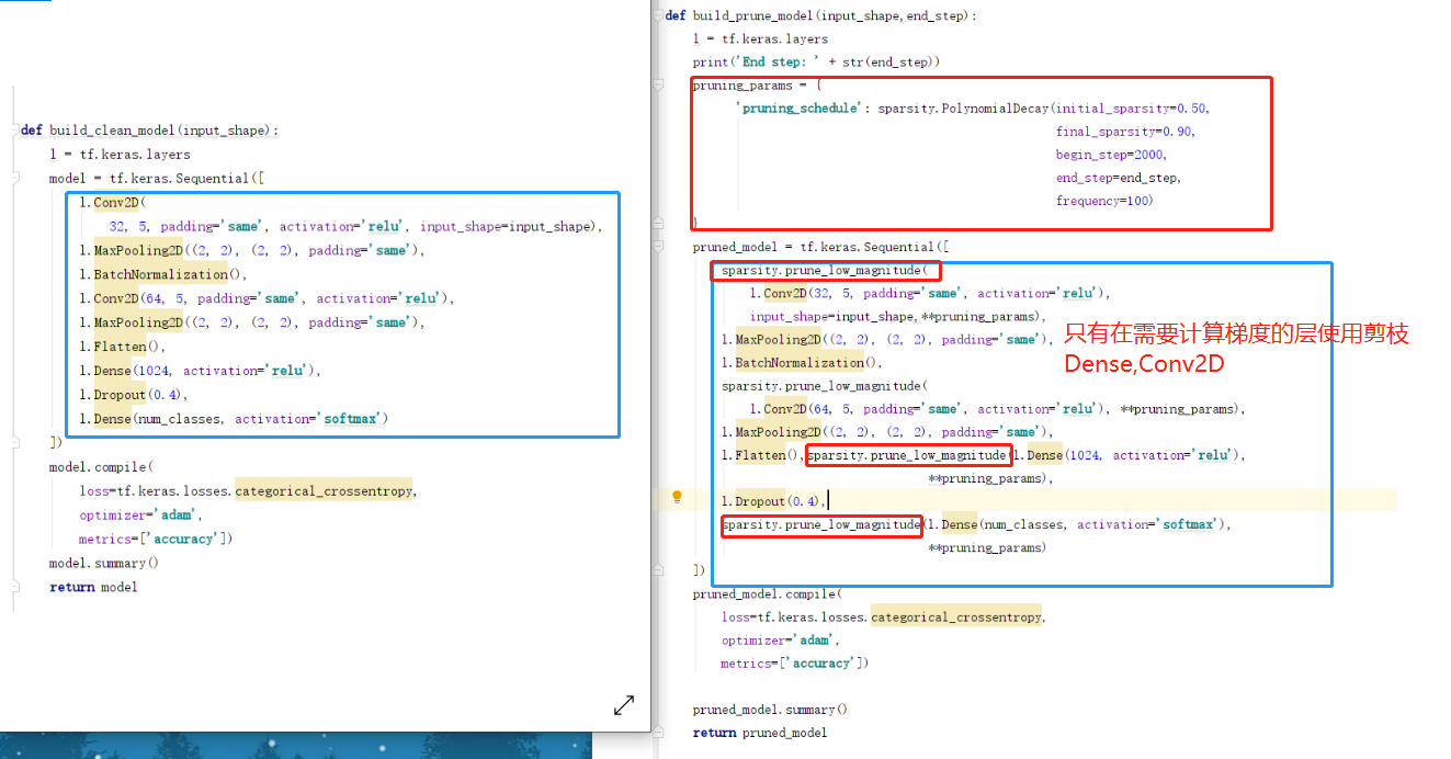
5.2.2 构建剪枝的MNIST分类模型 注意和上面的5.2.1构建原始分类模型的代码对比
1
2
3
4
5
6
7
8
9
10
11
12
13
14
15
16
17
18
19
20
21
22
23
24
25
26
27
28
29
30
31
32
33
34
def build_prune_model(input_shape,end_step): l = tf.keras.layers print('End step: ' + str(end_step)) pruning_params = { 'pruning_schedule': sparsity.PolynomialDecay(initial_sparsity=0.50, final_sparsity=0.90, begin_step=2000, end_step=end_step, frequency=100) } pruned_model = tf.keras.Sequential([ sparsity.prune_low_magnitude( l.Conv2D(32, 5, padding='same', activation='relu'), input_shape=input_shape, **pruning_params), l.MaxPooling2D((2, 2), (2, 2), padding='same'), l.BatchNormalization(), sparsity.prune_low_magnitude( l.Conv2D(64, 5, padding='same', activation='relu'), **pruning_params), l.MaxPooling2D((2, 2), (2, 2), padding='same'), l.Flatten(), sparsity.prune_low_magnitude(l.Dense(1024, activation='relu'), **pruning_params), l.Dropout(0.4), sparsity.prune_low_magnitude(l.Dense(num_classes, activation='softmax'), **pruning_params) ]) pruned_model.compile( loss=tf.keras.losses.categorical_crossentropy, optimizer='adam', metrics=['accuracy']) pruned_model.summary() return pruned_model
训练剪枝模型
1
2
3
4
5
6
7
8
9
10
11
12
13
14
15
16
17
18
19
20
21
22
23
24
25
26
27
def train_prune_model(x_train,x_test,y_train,y_test,epochs,prune_model_file): input_shape = (img_rows, img_cols,1) num_train_samples = x_train.shape[0] end_step = np.ceil(1.0 * num_train_samples / batch_size).astype(np.int32) * epochs pruned_model = build_prune_model(input_shape,end_step) # Add a pruning step callback to peg the pruning step to the optimizer's # step. Also add a callback to add pruning summaries to tensorboard callbacks = [ sparsity.UpdatePruningStep(), sparsity.PruningSummaries(log_dir=logdir, profile_batch=0) ] pruned_model.fit(x_train, y_train, batch_size=batch_size, epochs=10, verbose=1, callbacks=callbacks, validation_data=(x_test, y_test)) score = pruned_model.evaluate(x_test, y_test, verbose=0) print('Saving pruned model to: ', prune_model_file) # 保存模型时要设置 include_optimizer 为True by default. tf.keras.models.save_model(pruned_model,prune_model_file, include_optimizer=True) print('Test loss:', score[0]) print('Test accuracy:', score[1]) x_train,x_test,y_train,y_test = prepare_trainval(img_rows, img_cols) prune_model_file = "./prune_mnist_classifier.h5" train_prune_model(x_train,x_test,y_train,y_test,epochs,prune_model_file)
训练结果输出
1
2
3
4
5
6
7
8
9
10
11
12
13
52224/60000 [=========================>....] - ETA: 0s - loss: 0.0127 - accuracy: 0.9961 53120/60000 [=========================>....] - ETA: 0s - loss: 0.0126 - accuracy: 0.9961 54016/60000 [==========================>...] - ETA: 0s - loss: 0.0125 - accuracy: 0.9962 54912/60000 [==========================>...] - ETA: 0s - loss: 0.0124 - accuracy: 0.9962 55808/60000 [==========================>...] - ETA: 0s - loss: 0.0124 - accuracy: 0.9962 56704/60000 [===========================>..] - ETA: 0s - loss: 0.0123 - accuracy: 0.9962 57600/60000 [===========================>..] - ETA: 0s - loss: 0.0123 - accuracy: 0.9962 58368/60000 [============================>.] - ETA: 0s - loss: 0.0123 - accuracy: 0.9962 59264/60000 [============================>.] - ETA: 0s - loss: 0.0123 - accuracy: 0.9962 60000/60000 [==============================] - 4s 69us/sample - loss: 0.0123 - accuracy: 0.9962 - val_loss: 0.0226 - val_accuracy: 0.9920 Saving pruned model to: ./prune_mnist_classifier.h5 Test loss: 0.022609539373161534 Test accuracy: 0.992
如果我们要载入剪枝的模型,我们得使用prune_scope()会话
1
2
3
4
5
6
7
8
9
10
11
12
13
with sparsity.prune_scope(): restored_model = tf.keras.models.load_model(checkpoint_file) restored_model.fit(x_train, y_train, batch_size=batch_size, epochs=2, verbose=1, callbacks=callbacks, validation_data=(x_test, y_test)) score = restored_model.evaluate(x_test, y_test, verbose=0) print('Test loss:', score[0]) print('Test accuracy:', score[1])
在训练和载入剪枝模型时有两点需要注意
保存模型时, include_optimizer必须设置为True。因为剪枝过程需要保存optimizer的状态。
载入剪枝模型时需要在prune_scope()会话中来解序列化。
5.2.3 对照:如何使用剪枝模型 构建模型时
我们对比发现,只有需要计算梯度的网络层需要使用剪枝的包装。同时需要设定好剪枝的规划。
训练模型时
没有太大的区别,除了以下两点
需要新增关于剪枝的统计
保存模型时需要将optimizer也一起保存
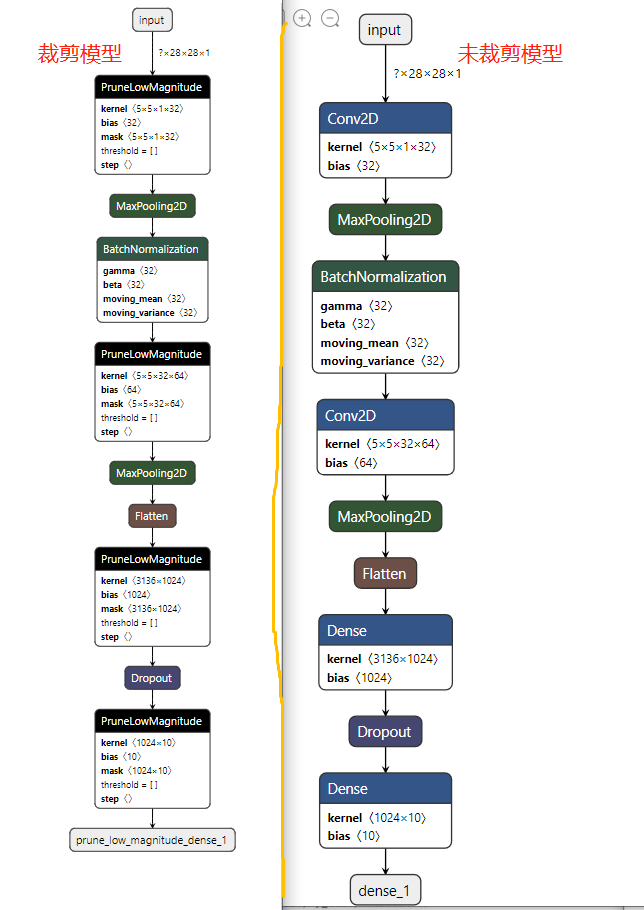
使用netron打开两个保存的模型,效果如下,可以看到裁剪的模型都被放在了PruneLowMagnitude中。
5.3 对整个模型剪枝 函数prune_low_magnitude可以应用于整个keras模型。此时算法会被应用于所有对权重剪枝友好 (Keras api的知道的)的网络层,不友好 的网络层会直接忽略掉,未知 的网络层可能会报错。
如果模型的网络层是API不知道如何剪枝的,但是非常适合不剪枝,那么交给API来修剪每层的basis即可(即不修剪卷积核的权重,只修剪basis)。
除去剪枝配置参数,相同的配置可以应用于网络的所有的剪枝层。同时需要注意的是,剪枝不保留原模型的优化器optimizer,需要对剪枝的模型重新训练一个新的优化器optimizer。
开始之前,假设我们已经有一个已经序列化过的预训练的Keras模型,想对其权重剪枝。以前面的MNIST模型为例。先载入模型
1
2
# Load the serialized model loaded_model = tf.keras.models.load_model(keras_file)
然后可以剪枝模型然后编译剪枝之后的模型并训练。此时的训练将重新从第0步开始,鉴于模型此时已经达到了一定的准确率,我们可以直接开始剪枝。将开始步骤设置为0,然后只训练4个epochs。
1
2
3
4
5
6
7
8
9
10
11
12
13
14
15
16
17
epochs = 4 end_step = np.ceil(1.0 * num_train_samples / batch_size).astype(np.int32) * epochs print(end_step) new_pruning_params = { 'pruning_schedule': sparsity.PolynomialDecay(initial_sparsity=0.50, final_sparsity=0.90, begin_step=0, end_step=end_step, frequency=100) } new_pruned_model = sparsity.prune_low_magnitude(model, **new_pruning_params) new_pruned_model.summary() new_pruned_model.compile( loss=tf.keras.losses.categorical_crossentropy, optimizer='adam', metrics=['accuracy'])
再训练4个epochs
1
2
3
4
5
6
7
8
9
10
11
12
13
14
15
16
17
# Add a pruning step callback to peg the pruning step to the optimizer's # step. Also add a callback to add pruning summaries to tensorboard callbacks = [ sparsity.UpdatePruningStep(), sparsity.PruningSummaries(log_dir=logdir, profile_batch=0) ] new_pruned_model.fit(x_train, y_train, batch_size=batch_size, epochs=epochs, verbose=1, callbacks=callbacks, validation_data=(x_test, y_test)) score = new_pruned_model.evaluate(x_test, y_test, verbose=0) print('Test loss:', score[0]) print('Test accuracy:', score[1])
模型导出到serving
1
2
3
4
5
6
7
8
9
10
11
12
13
14
15
16
final_model = sparsity.strip_pruning(pruned_model) final_model.summary() _, new_pruned_keras_file = tempfile.mkstemp('.h5') print('Saving pruned model to: ', new_pruned_keras_file) tf.keras.models.save_model(final_model, new_pruned_keras_file, include_optimizer=False) # 压缩之后的模型大小与前面一层层剪枝的大小一样 _, zip3 = tempfile.mkstemp('.zip') with zipfile.ZipFile(zip3, 'w', compression=zipfile.ZIP_DEFLATED) as f: f.write(new_pruned_keras_file) print("Size of the pruned model before compression: %.2f Mb" % (os.path.getsize(new_pruned_keras_file) / float(2**20))) print("Size of the pruned model after compression: %.2f Mb" % (os.path.getsize(zip3) / float(2**20)))
参考
medium Pruning Deep Neural Networks tensorflow mnist 剪枝 Pruning deep neural networks to make them fast and small stackoverflow 如何在tensorflow计算梯度时更改计算方式 Tensorflow官方API 如何更改梯度计算方式